High Precision Frequency Counter using GPS (Part2)

Following from previous posting I have connected a STM32F429i-DISC1 board to us UBLOX NEO-6M GPS module (see https://www.ebay.co.uk/itm/313603433572) and programmed a 32 bit counter in capture compare mode running at 80MHz.

STD32f429i-Disc1 with NEO-6M GPS as timer — NEO-6M GPS with PPS triggering counter

After the GPS settled I recorded a number of counts varying by +-200 using the inbuilt 8MHz crystal.

This is far too much jitter, at present i t is uncertain if the reason is

Crystal frequency variation due to quality of crystal
Crystal frequency variation due to supply voltage
STM32 PLL stability.

I will first attempt to attach a better crystal. The STM32F429 accepts an external input from 4MHz to 26MHz. From RS components I considered a 24Mhz TCXO https://uk.rs-online.com/web/p/tcxo-oscillators/2499379 but I only wanted one, so ended up buying o e of these from ebay https://www.iqdfrequencyproducts.com/products/pn/LFTCXO075797Reel.pdf.

I’ll update on stability when it arrives.

I will provide the eclipse project for the board firmware. It includes UI, GPS serial communications and timer programming. All running under FreeRTOS.

High Precision Frequency Counter using GPS

To recalibrate my ageing HP 3850A spectrum analyser I needed a 6 digit frequency counter. After looking at buying a used device I realised that the purchase and calibration would cost me £300 plus, and constant recalibration would be required.

I had a STM32F407 controller laying around, and a MBLOX GPS module, and wondered if the PPS (pulse per second) signal could be used to provide an accurate frequency reference and I could create a decent frequency counter based on this?

Using a 32 bit counter synchronised by the PPS GPS signal, we can get an accurately calibrated count. Using clever software we can use the initial count value, and could average readings to further improve accuracy.

From the MBLOX data sheet the PPS signal is accurate to 30nS, this is 0.06 parts per million (ppm) giving a good 7 digits accuracy.

The two measurement techniques are:

Use a calibrated counter and trigger reading on rising/falling edge of incoming signal, for frequencies below a suitable break point (TBD).
Count incoming pulses and use PPS to get count, the upper frequency is limited to the maximum counter speed.

Triggering on edge of incoming signal

Measuring a 20KHz signal using with a 80MHz counter clock would give a count of 4,000 initially, giving 3.5 digits accuracy, but averaging over 100 counts would give 4,000.00, 6 digits accuracy. This would only take a 1/200th of a second. Averaging over 1000 counts would happen in a 1/20th of a seconds giving 4000.000 6.5 digits accuracy.

40KHz would give a count of 2,000, but if counting for 1 second we got 40,000 in a second, which is far slower. The averaging technique can be used, resetting if there is a significant frequency change up to about 50 KHz.

Choice of board

STM32F407 on the STM disc-1 development board has a LCD display and USB, and two 32 bit counters. TIM 2 and TIM 5. These have a maximum clock of about 80MHz. The touch display would allow user input configuration to be trivial. I picked up my development board for £32 – bargain. All that would be required is a small case, input filtering and buffering of the measured source and attachment of the GPS receiver.

It may be necessary to use an external GPS antenna TBD. See part 2…

Ultra Low Distortion HiFi VAS Amplifier stage

To build a low distortion (up to 20KHz) and high output power amplifier requires a ultra low distortion, low impedance output stage with an open loop gain exceeding 1MHz.

To realise such a design, and keep the noise figure as low as possible a large number of design considerations have been considered until a viable design (tested using SPICE simulations) is proposed. This work has taken years of thought and months of simulation and redesign.

The output stage will use MOSFET devices as opposed to bipolar, this has been chosen for the following reasons:-

The inherent Rds limits the short circuit current sufficiently to permit the use of an external short circuit protection circuit to be used that does not contribute to amplifier distortion.
The negative temperature coefficient of MOSFET simplifies the design of a thermally stable output stage.
The higher frequency response permits a tighter feedback loop further reducing distortion.

Bipolar devices are capable of delivering equivalent performance, but with additional complexity, this often is at the expense of non linear audio distortion. Years of listening to bipolar vs MOSFET designs has proved MOSFET’s sound better, although MOSFET devices are more expensive, often require higher idle bias current and are harder to source.

The MOSFET output topology has been carefully considered and over 20 alternate topologies tried, some offer considerable cross over distortion reduction but at the price of difficult driving impedance or poor thermal stability. After months of experimentation, electrical and thermal modeling it has been decided to return to a traditional source follower approach.

Low Noise FET Input

The use of a FET input stage greatly reduces DC offset as it is a voltage amplifier as opposed to current hence input bias currents do not affect DC offsets. The matching of the input FET devices is aided by matched pairs, for this reason the LSK389 has been a popular choice. Sadly the high capacitance of the input, around 20pF greatly limited phase and frequency responses. 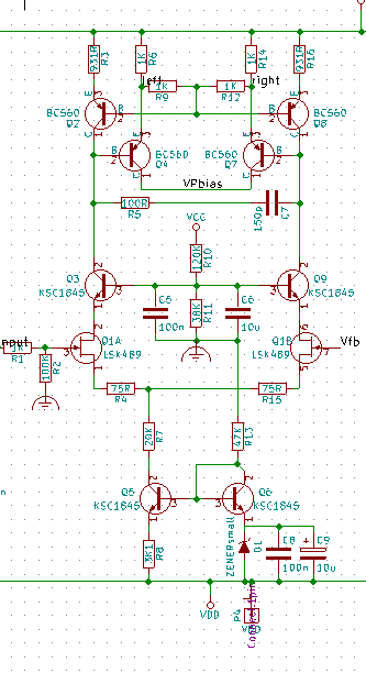The newer LSK489 is an ideal choice with only 4pF capacitance and $4.7uV/\sqrt Hz$ noise and superb Vgs matching reducing offset voltage errors, please refer to Bob Cordell’s LSK489 application note for more information.

The use of a temperature compensated constant current sink and cascaded FET drains yields the following differential topology:-

The voltage source is a low noise temperature compensated zenor device at 6.2V. This provides a 2mA sink current through R7. The power rails are +-60V, so the voltage on the source of the LSK489 devices is approximately $60 - (6.2V + 0.6V + 0.002mA * 20000 \Omega)$ , -13.2V. Transistors Q3 and Q9 act as cascade to the LSK489 differential pair and reduce the voltage across the LSK489 device to:-

$38000 \Omega * 60V / (120000 \Omega + 38000 \Omega) -0.6V = 13.8V$

This places a maximum voltage of 27V across LSK489 – Well within it’s design parameters.

The filtering across the reference Zenor diode here is non optimal, the output impedance of the noise across D1 is low and should has a series resistor to reduce noise.

R5 and C7 place a pole at around 3MHz, limiting the differential bandwidth. The final design has a number of zero’s and poles to stabilize the amplifier and produce a favorable bode plot.

The cascoded FET stage also acts to reduce the voltages across the top current mirrors and low impedance drivers Q2, Q4, Q7 and Q8 which can be a very low noise, high frequency bipolar device. BC560C‘s were chosen here as they have suitable high gain.

Care was taken to match transistors in equal gain pairs, although the emitter degeneration reduces the effect of this.

HiFi Amplifier Thermal Design Considerations

When designing ultimate high fidelity audio amplifiers thermal stability and cooling become a huge issue. Here I consider a design of a class AB amplifier with a MOSFET output driver stage.

The amplifier is designed to deliver approximately 100W undistorted, this will require a +-45V supply rail. To drive the MOSFET’s a higher supply voltage is required. In this design I have chosen 55V, the driver stage draws 19mA, equating to 2W of power per channel. In addition the output MOSFET’s will require a residual bias current of 60mA, consuming 5.4W. This amounts to 7.4 watts idle per channel, 15W in total at idle.

There is little we can do to reduce this, clever standby logic can reduce this by disabling the output driver when no signal is present, but when in use, and when under a 20W load for example 30W of heat will need to be dissipated.

Passive cooling is preferred over fan noise, an almost perfect high fidelity system be pointless if a fan is producing noise in the background. Passive cooling is vulnerable to poor airflow so thermal monitoring and shutdown is mandatory in such systems to ensure when, for example a record sleeve is placed over the amplifier it does not overheat.

The thermal stability of the output stage also needs careful design, in classical MOSFET output stages the idle bias current is chosen to be the point at which the device is thermally stable. An example of this are the Exicon ECX10N20 devices (see datasheet) where the Vgs temperature coefficient is zero at 110mA and increases beyond this point. Sadly 110mA is far too high, so additional temperature compensation is required to stabilize the devices at a lower idle bias point. The negative temperature coefficient at higher currents protects against short circuit and high temperature failure making these devices extremely rugged:-

Exicon Bilateral MOSFET Vgs vs Temperature

Using such devices has yielded classical MOSFET amplifier designs which have passed the test of time. An Hitachi power MOSFET design was included in their design guides in 1985 which was the basis of the Maplin Electronics 75W amplifier:-

I built a pair of similar amplifiers which sounded great and were bomb proof, continuing to work for over 20 years.

A similar output stage, which turns a current source into a bias voltage that is thermally stable is shown below:-

Simple Current to Voltage Source Follower MOSFET output

Transistor Mounting

The heat-sink will have a cooling ability defined as a thermal resistance ( $^{\circ}C/W$ ). This can only be achieved if the transistor junction is perfectly thermally coupled to the heat-sink.

Unfortunately there are other thermal resistances between the actual transistor junction and the heat-sink, which can be reduced to a transistor junction to case resistance and a case to heat-sink resistance:-

heatsink mounted transistor thermal model — Thermal Model of Heatsink mounted Transistor

The thermal capacitance $C_j$ is small compared with $C_{case}$ , but the value of $R_{th}$ for the junction to the case is fairly large. It is important to reduce the value of the thermal resistance between the case and heat-sink to maximise the heat-sink capacity.

The table below shows the typical thermal resistance of different materials:-

Material	Electrical Insulation	Thermal Resistance Wm-1°C-1	Cost	Notes
Mica	4500 volts/mm	0.528	High	Requires silicon paste
Sil-Pads	700 volts/mm	1.0	Medium	Easy to use
Kapton		0.9-1.5	High	Ages under high temperatures

Kapton is used in many designs, but suffers with lower thermal conductivity and stability over time. Using mica with thermal compound is expensive, difficulty and messy, but is the best solution. For ultimate high fidelity designs we will use mica washers and thermal compound.

Care must be taken not to contaminate any connections with silicon thermal compound as (i) it prevents reliable soldering and (ii) it eventually leads to connector failure if contaminating any connectors.

The final piece of the puzzle is the use of a Vbe multiplier to set the MOSFET bias point. This design has been used in most high fidelity amplifiers to provide some -Ve thermal compensation into the output stages and allow the bias voltage to be easily adjusted:-

Vbe Muliplier — Vbe Multiplier (Bias servo)

Often R1 or R2 is variable to adjust the bias point of the output FET’s and the transistor is bolted to the output heat sink close to the output devices. The Vbe offset voltage drops as temperature rises ensuring voltage Vce is inversely proportional to the temperature.

The use of a variable resistor for r1/r2 vastly affects reliability and can contribute towards distortion caused by non linear effects in carbon tracks. It is often better to use a select on test approach using fixed metal film resistors. This approach has been adopted in this design.

Finally, the choice of heat sink material is to be considered. It is clear that copper is a far better conductor of heat:-

Thermal Conductivity of Metals

Material	Thermal Conductivity $Wm^{-1}K^{-1}$	Notes
Aluminium	237	Surface oxidation also increases contact resistance
Copper	401	Copper is rarely 100% pure - so often this figure is slightly smaller
Steel (carbon 1%)	43

This table compares the thermal conductivity of common metals used in electronic equipment

From here copper seems ideal. In this design a large copper plate will conduct heat away to the chassis which will be covered in a large aluminium heat sink. Aluminium is far stronger and easier to machine into complex heat sink shapes.

MOSFET High Fidelity Output Stage

There are countless publications and designs for high-fidelity audio power amplifiers. As an audio engineer I have recently been designing a new power amplifier to replace my 3rd generation amplifier initially built over 25 years ago.

Class AB amplifier using Hitachi Lateral MOSFETS

Much discussion has been made on “Square Law” and “Cube Law” amplifiers to reduce harmonic distortion by altering the drives to the output devices.

As an initial study, I simulated the following circuit in LTSpice and extracted a polynomial regression of the input and output data points. This then gives a clear indication of the transfer function. The following circuit:-

bipolar_mos_op — Bipolar Transistor driving MOSFET output

Running a spice simulation followed by a 5th term polynomial regression yielded the following equation:-

$1.0371786 + 5.0875544x + 0.22985048x^2 -0.05428182x^3 + 0.005091393x^4$

The 1.03 offset is unimportant, the 5.09 is the gain of the stage. The unwanted components are the square, cube and quadratic terms. The higher order terms produce greater distortion at higher signal amplitudes.

It is worth comparing this with the equivalent circuit using a MOSFET driver:-

output_fet_fet — MOSFET Output stage driving EXICON Lateral MOSFET

This produced the following polynomial:-

$0.67743263 + 5.1414499x 0.14129363 x^2 -0.0204953^3 +0.0011353254x^4$

Clearly the $x^2$ term is smaller as expected, but in addition the $x^3$ and $x^4$ terms are smaller. If we further reduce the gain to 2, by adjusting the feedback resistors we get:-

$0.4495991+ 1.8448146x + 0.028082105x^2 -0.0040223748x^3 +0.00022303229x^4$

If we can alter the drive to have -ve $x^2$ and $x^3$ terms we should be able to reduce distortion considerably. The largest distortion contribution is the $x^2$ component.

This work progressed to analysing hundreds of MOSFET output stages, the best design based on work suggested by Bob Cordell in his book Bob Cordell “Designing Audio Power Amplifiers”

This design has very low THD, but required additional complexity to the driving VAS stage. The distortion improvements in the output stage were lost in the additional complexity in the VAS driving stage.

The final decision was to use a conventional source following design with 3 pole miller compensation and careful VAS design. Most distortion is generated at +-1V where there s a transconductance imbalance. The initial design will ignore this and allow the feedback to cancel most of this error. The snag with -Ve feedback is it’s performance at higher frequencies, if the frequency response of the VAS stage is insufficient the error at 20KHz will be greater. We will consider the use of local error injection into the driver stage to reduce this error, hence reducing high frequency distortion.

Caching name service to improve unix server stability

Introduction

Over the past few years I’ve seen a number of cases where Unix systems have suffered serious outages caused by the loss of a primary name server. Such systems appear really slow, and often when used in conjunction with Samba or a remote name service such as Centrify servers may appear to hang.

The main reason for this is the manner in which Unix performs DNS lookups, by first looking at the primary name server, then trying the secondary etc. Since it is stateless, a successive lookup will hit the primary server before trying the second, even if it is not responding. Loss of the primary name server will cause all programs making a remote connection via hostname (not IP) will experience a DNS timeout delay before connecting.

On machines with a reasonable degree of DNS lookups, this eventually consumes a large amount of system resources as requests block and accumulate, and in some cases has resulted in servers running out of physical memory.

Name Service Caching Daemon

One solution is to use a name service caching daemon, there are a number available, and many Linux distributions include prepackaged solutions. Care must be taken to fully understand how these programs operate as they are often implemented lower in the service stack.

Using a bind cache to reduce the problem…

The simple and reliable solution is to install a local caching name server, a simple lightweight bind install configured to forward requests to the primary and secondary (and other) name servers, but only listening on localhost, and with zone transfers etc disabled for security reasons. Then the nameserver 127.0.0.1 is added to the servers /etc/resolv.conf to ensure it’s used. As bind obeys “time to live” cache times, there is no impact on name resolution accuracy.

On failure of a primary name sever, the local caching name will cache the secondary name server response, so successive lookups of the same address will return instantly. In addition most lookups will already be cached, hence temporary loss of the primary name server often goes unnoticed.

Caching Bind Config

The named.conf file for bind is shown below, the forwarders section should contain the list of name servers from the /etc/resolv.conf, the resolv.conf file should have name server 127.0.0.1 added before the other name servers.

options {

    listen-on { 127.0.0.1; };

    directory "/var/named";

    dump-file "logs/named_dump.db";

    forwarders {

        //  LOCAL-FORWARDERS

    };

    forward only;

};

 

logging {

    channel "mainlog" {

    file "logs/named.log" versions 3 size 1m;

    print-category yes;

    print-severity yes;

    print-time yes;

};

channel "querylog" {

    file "logs/query.log" versions 2 size 1m;

    print-category yes;

    print-severity yes;

    print-time yes;

};

category queries {

    //  Uncomment next line to log query messages.

     #querylog;

    null;

};

category default { mainlog; };

};

Bigmite creating software and hardware solutions….

Chroot sftp using openssh and logging

Introduction

I have seen many posts on how to set up chroot jail’ed sftp using openssh, but few cover the logging aspects in detail. This tries to cover some of the issues and solutions.

SFTP

SFTP is ftp wrapped in a SSH secure environment. It is used to transfer files securely and is now used widely to transfer files between servers securely. Open SSH is the most common ssh implementation and includes all the required configuration logic to allow group based access control and chroot jail’ing of users.

Chroot Configuration

In this example I am going to set up a group of users that require SFTP access only (no SSH) and are going to copy files to a filesystem on a SFTP server. The location of the filesystem is going to be /sftp and users will reside in seperate folders under here.

Initially a new group should be created, here called “sftpuser”. Each user that requires SFTP access will be placed in this group.

The sshd_config (on debian in /etc/ssh) should be edited and the following added on the end:-

Match group sftpuser
 ChrootDirectory /sftp/%u
 X11Forwarding no
 AllowTcpForwarding no
 ForceCommand internal-sftp -l VERBOSE -f LOCAL6

This does the following:-

Forces all users connecting via ssh on port 22 to have sftp only
Runs their sftp session in a chroot jail in directory /sftp/$USER
Prevents them TCP of X11 forwarding connections
Runs the internal sftp server getting it to log verbose and to syslog channel name LOCAL6

Now a user should be created, without creating a home directory and in the default group sftpuser. On ubuntu you can enter:-

adduser --home / --gecos "First Test SFTP User" --group sftpuser --no-create-home --shell /bin/false testuser1

The reason the home directory is set to / is that the sftp will chroot to /sftp/testuser1. Next the users home directory will need creating:-

mkdir /sftp/testuser1
chmod 755 /sftp/testuser1
mkdir /sftp/tstuser1/in
mkdir /sftp/testuser1/out
chown testuser1 /sftp/testuse1/in

Note that the directory structure and permissions that you set may differ depending on your requirements. The users password should be set, and sshd restarted (on debian service ssh restart).

Now it should be possible to sftp files to the host using the command line sftp tool, but it should not be possible to ssh to the server as user testuser1.

Logging

You will see verbose sftp logging being produced in the /var/logmessages for each chroot’ed user, where by default this should go to the daemon.log. The reason for this is that the chroot’ed sftp process can not open /dev/log as this is not within the chrooted filesystem.

There are two fixes to this problem, depending on the filesystem configuration.

If the users sftp directory /sftp/user is on the root filesystem

You can create a hard link to mimic the device:-

mkdir /sftp/testuser1/dev
chmod 755 /sftp/testuser1/dev
ln /dev/log /sftp/testuser1/dev/log

If the users sftp directory is NOT on the root filesystem

First syslog or rsyslog will need use an additonal logging socket within the users filesystem. For my example /sftp is a seperate sftp filesystem.

For Redhat

On redhat syslog is used, so I altered /etc/sysconfif/syslog so that the line:-

SYSLOGD_OPTIONS="-m 0"

reads:-

SYSLOGD_OPTIONS="-m 0 -a /sftp/sftp.log.socket

Finally the syslog daemon needs to be told to log messages for LOCAL6 to the /var/log/sftp.log file, so the following was added to /etc/syslog.conf:-

# For SFTP logging
local6.*                        /var/log/sftp.log

and syslog was restarted.

For Ubuntu Lucid

On Ubuntu lucid I created /etc/rsyslog.d/sshd.conf containing:-

# Create an additional socket for some of the sshd chrooted users.
$AddUnixListenSocket /sftp/sftp.log.socket
# Log internal-sftp in a separate file
:programname, isequal, "internal-sftp" -/var/log/sftp.log
:programname, isequal, "internal-sftp" ~

… and restarted rsyslogd.

Creating log devices for users

Now for each user a /dev/log device needs creating:-

mkdir /sftp/testuser1/dev
chmod 755 /sftp/testuser1/dev
ln /sftp/sftp.log.socket /sftp/testuser1/dev/log

Log Rotation

TBD

Producing xfer logs

The format of the logging from openssh’es sftp server is a little cryptic. The perl script here can be used to produce an proftp like xfer log. Bigmite Software Solutions are experts in finding simple solutions to everyday problems.

Several people have said they had trouble running the script to produce Xfer logs. I’ll try to write a wrapper for ubuntu logroate and redhat later, but for now:-

Save script somewhere sensible and run “chmod +x createXferLog”, then to create a Xfer log from another log file simply type:-

createXferLog logfile > xfer.log

The file will be the syslog, or daemon log depending on system, the file with sshd logs in,

cat logfile | createXferLog > xfer.log

Poll, Push or Pull – Which is best….

What do we mean by “Poll”, “Push” and “Pull” in terms of data communication

Communications systems either “Push” or “Pull” data, but in some cases, when you need to know if anything is waiting a “Poll” is performed, these techniques each have advantages and disadvantages discussed here.

Polling

Polling is asking whether data is available, or can be sent, for example the pop3 protocol used by main readers. It is very simple and has the advantage that the server being polled need not know anything about the polling client state. The polling client must make periodic requests to the server to determine if data is ready or can be sent.

The disadvantages of “Polling” are that the polling client will not know exactly when it can send or receive data, hence to reduce latency the poll interval may need to be quite frequent increasing the server overhead, especially if it serves a number of clients.

If the polling interval is set to n, and the data transfer time m, then the average delivery/fetch latency is n/2 + m. This can be a limit in many systems.

Computer hardware has historically suffered from issues where some hardware did not use interrupts to indicate data reception, or, like in the PC the old interrupt controller having limited interrupts caused devices to share an interrupt. This in turn increased interrupt latency as the IBM PC had to poll all the hardware devices sharing this interrupt to determine the interrupt source. Hence the evolution of the APIC.

Polling is a solution only to used where servers need not know availability of clients, low latency is unimportant and the host being polled is able to handle the amount of polling requests.

Examples of services using “Poll” are NTP, POP3,

Pushing

Pushing of data is highly efficient and is where a host pushes data to the receiving host. Many protocols use such schemes such as:-

Cups (Printed files are pushed to print server)
FTP (oddly uses “Pull” as well) (files are ushed to remove server)
LPR (Printed files are pushed to print server)
SFTP (Secure FTP using ssh wrapper)
SNMP (Simple Network Messaging Protocol)
SMTP (Internet email delivery – very old – very reliable)
Hardware Interrupts

“Pushing” is best used where data is ready for delivery and the client can accept data at any time.

Double Buffering

In some cases, such as writing large amounts of data to a “block” based piece of hardware, double buffering can be used to vastly reduce latency.

Consider a network adapter, which has an output buffer, and interrupts when it has completed a transmit. The OS writes a packet of data to the buffer, then waits for the card to send the data. When the hardware has successfully send the data it interrupts the OS to inform that it is ready to receive more data, but the time taken for the OS to service the interrupt filling the transmit buffer may delay a successive network transmit, adding unwanted delay between packets.

The solution is to utilise two transmit buffers in the hardware device, buffer a and b. Following successful transmission of buffer a, the network adapter will start to tranmit the data in buffer b (if ready) as well as interrupt the computer to instigate a data copy to buffer a. This ensures that the delay following the interrupt and the OS copy of data to buffer a does not add additional latency to the system. The OS software requires little change to cater for this type of system, but the throughput gains are massive. The overall latency of the system is not reduced, but the throughput is increased.

Pulling

Pulling of data is done when a client requires data, and is normally served by fast services. Most client user interfaces use “Pull” type services to achieve the fast response expected by a user. Examples of such services are:-

FTP
HTTP (driving the internet)

The HTTP protocol is a best use case, where users pull content “On Demand” and has driven the last 20 years of Internet development.

Conclusion

Most data communications systems work best when “Pulling” or “Pushing” data, the use of a “Poll” type system should be avoided unless their is a clear business case.

When designing systems it’s often simpler to implement a scheme which works “Sufficiently Well”, but if designed inappropriately requires more resources and power. It is often possible to implement systems that utilise very few resources by careful interface designs, and for low power embedded devices this is so important.

High Performance Hosting – Unfinished

Introduction

Over the years I’ve been asked to produce a number of high reliability high throughout web hosting solutions. Although there are a number of off the shelf solutions that are expensive, the true high availability solutions can be realised using standard linux builds.

In the following article I’ll outline aids to help you build low cost HA solutions using linux.

Load Balancing

For high throughput application it is often not possible to host on a single server. In addition the availability of a single host cannot be guaranteed, so a multi hosted solution is often better.

Developing web applications that can run on multiple servers poses a number of problems, mainly around state maintenance and session management, but these will be covered elsewhere.

Commercial Load Balancers

Commercial hardware load balancers offer a range of features, but you must always consider the “Single Point of Failure” problem, even if the load balancer has dual power supplies etc it can fail, or require replacement. It is always better to buy two complete units that can work in parallel offering higher availability. Upgrading a single unit can be done without fear of loss off service.

By using an external pair of round robin DNS entries it is possible to spread the load across balancers. In the event of a balancer failing you can move the failed IP address to the remaining balancer.

Commercial load balancers are expensive!.

Linux Load Balancers

Using two linux servers and a high availability heartbeat configuration provides a far cheaper solution had has been used by Bigmite Hosting Solutions. Using two linux servers in a HA configuration and running suitable load balancing software a high throughput can be achieved.

A small server can saturate a 1Gb/s network link, leaving the back end application servers to do the work. The choice of load balancing software depends on your requireements such as:-

Session Management
Keep Alives
Monitoring
Latency

If no session management is required (such as a static site) then the kernel based ipvs (Linux Virtual Server) can be used, this is part of the standard linux distribution, and is simple to configure and very reliable.

If sessions need to be maintained to a client then layer x based load balancing is required. Packages such as HAProxy and BalanceNG (which is next generation of the balance software) offer these features.

Heartbeat

Heatbeat (www.linuxha.org

Requests for comments……

It is NOT finished…. it’s just ready for comments…. I’ve two busy to complete – please comment, and I’ll add your comments…..

Low Power Computers

In our office we have a development machine which runs all our websites in development along with a number of other applications. This computer is powered 24/7 and consumed considerable energy. The plan was to build a new faster machine that used a fraction of the energy.

The requirements were large storage (1T byte), 4G ram, capability to drive a large DVI panel for developers and a large number of USB ports. In addition we used an ADSL router which itself consumed 8 watts so using an ADSL USB model plugged into this machine would save further energy. Originally the server had raid disks, but the choice was made to backup regularly and use a single disk to save energy.

It’s worth noting that units using small power adapters have poor load factors and even if they consume a small amount of energy the effective transformer losses at the local substation due to poor load factors increase losses – so eliminating additional system components saves more energy than you expect.

The chosen components were:-

ASUS AT3N7A-I motherboard – this is a dual core atom motherboard with a nvidia ION chipset providing exceptional graphics (DVI connector) and low power consumption. In it’s mini-itx form factor it also reduces space requirements.
ST31000528AS Seagate 1TB SATA HDD – This is the seagate low power version, and performed better than expected.
4G Kingston RAM – Chose a manufacturer that offered a lower power device, there is a vast variation in power consumption of memory devices.
Noah Mini-ITX Case – Silver/Black – this case had in integral DC-DC adaptor and required no additional fans. It was strongly constructed and had a range of front panel connectors.
Speedtouch 330 USB Modem – this modem is a third generation speedtouch modem, and is well supported in linux and consumed minimal power.
Ubuntu Linux OS – I’m a Unix developer, so using windows would have been madness – but Unix has a smaller memory footprint and lower CPU utilisation on average. In addition it’s easier to run a large number of Unix applications in parallel than on a Windows system as the library loading, and configuration file separation facilitate better isolation of applications.

Low Power Server — New Low Power Office Server

Most of these components were purchased from LinITX in the UK who helped with the case choice.

The large number of cables feed all the office printers, scanners etc along with the USB ADSL modem.

Further power savings were made by turning off all unused devices (printers scanners etc).

The final power consumption was less than 35 watts, which considering how much work this machine is doing is remarkable. It is running ubuntu Karmic, awaiting the release of 10.04 LTS (the 8.04 version did not support the new nvidia graphics properly out of the box).